The Math of Scaling: Why Fluid Budgets Outperform Static Plans in the Algorithmic Era
A static budget is not a plan. It is a liability.
The organizations that treat ad spend as an administrative function, fixed during quarterly planning and adjusted annually at best, are systematically losing ground to operators who reallocate capital in response to real-time performance signals. The mechanism of the loss is predictable: rigid budgets trap spend in channels that have hit their efficiency ceiling while leaving high-growth opportunities unfunded because the capital was allocated elsewhere before the opportunity appeared.
The algorithmic era made this problem worse, not better. Google's machine learning systems require a specific data density threshold to function reliably. When budgets are too conservative to provide that density, campaigns stall in extended learning phases. When budgets are too inflexible to shift when a channel saturates, average ROAS holds steady while marginal returns crater below break-even. The dashboard looks acceptable. The last dollar spent is losing money.
Competitive discipline in this environment does not mean spending more. It means ensuring that every dollar is allocated to its highest marginal return in real time, and that allocation shifts as performance signals change.
For the account-level signal architecture that makes budget decisions meaningful, The $1,127 Algorithmic Tax covers why the conversion data underneath your budget decisions determines whether those decisions are based on reality or noise.
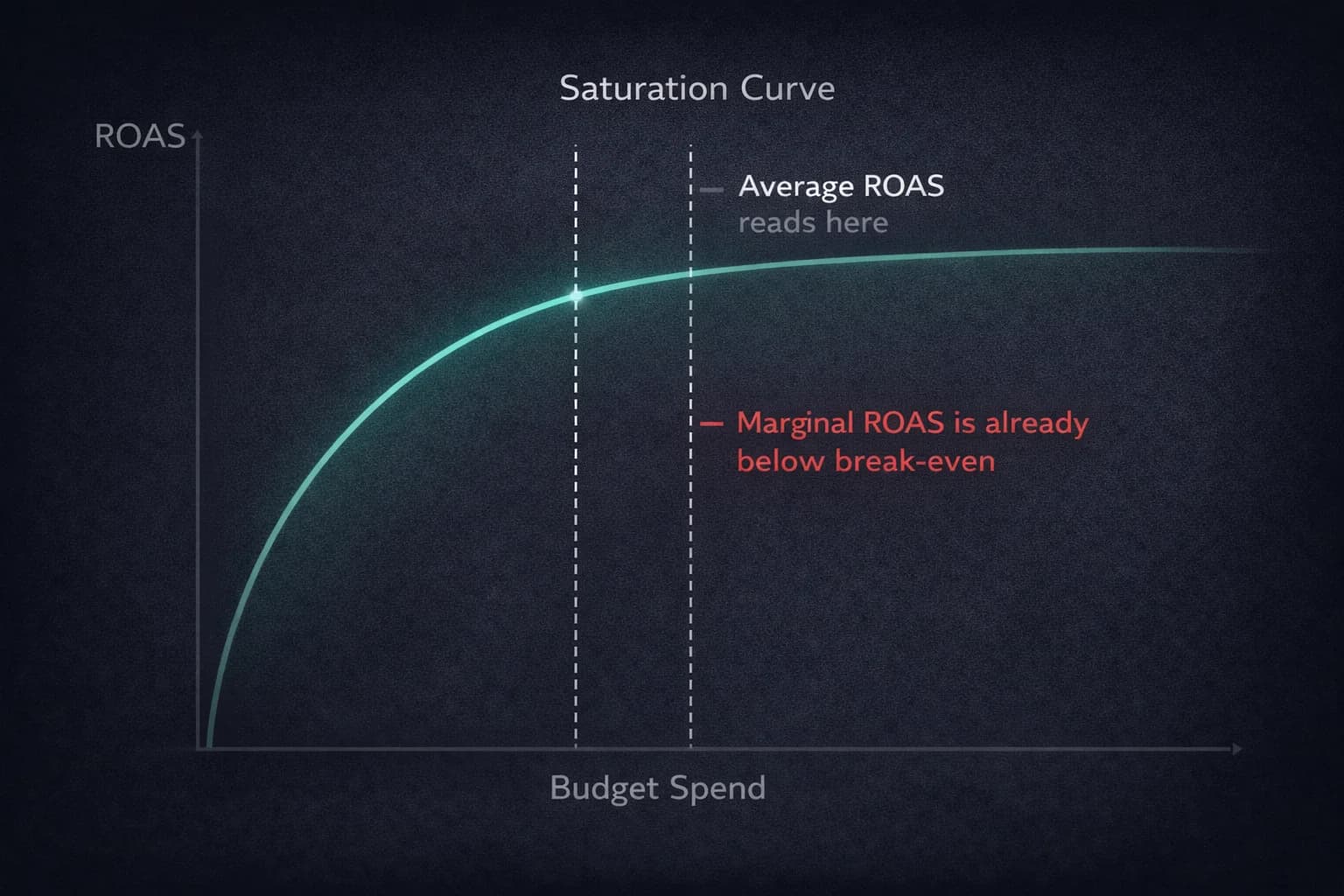
Average ROAS vs. Marginal ROAS: The Metric That Reveals the Efficiency Ceiling
The most dangerous number in a Google Ads report is a healthy average ROAS on a saturated campaign.
Average ROAS is a historical health check. It tells you the aggregate return on everything you have spent. It says nothing about what the next dollar will return. In hundreds of account audits, the pattern that appears most consistently is an account maintaining a respectable 3.5 average ROAS while the marginal return on the last $10,000 spent has dropped to 1.8, well below break-even for most businesses.
The advertiser sees 3.5 ROAS and increases budget. They are actually scaling losses.
| Average ROAS | Marginal ROAS | |
|---|---|---|
| Definition | Total revenue divided by total spend | Additional revenue generated by the next dollar spent |
| Utility | Historical efficiency reporting | Diagnostic tool for identifying the efficiency ceiling |
| Focus | Hides saturation | Reveals the point of diminishing returns |
| Scaling risk | Can stay high while incremental spend loses money | Signals exactly when to reallocate capital |
The saturation curve explains why this happens. Every campaign exhausts its most responsive audience segments first: the high-intent users who were already looking for what you sell. As budget increases, the algorithm reaches progressively less responsive segments. Conversion rates fall. CPAs rise. Average ROAS declines slowly because it is diluted by all the efficient earlier spend. Marginal ROAS falls faster and more honestly.
Tracking marginal ROAS requires segmenting your performance data by spend increment over time, not just looking at totals. A simple approach: pull weekly performance data and calculate the ROAS on each incremental spend increase. When marginal ROAS falls below your break-even threshold, that campaign has hit its efficiency ceiling and additional budget belongs elsewhere.
Building the Single Source of Truth
Dynamic budget allocation is impossible on broken data. Browser-based conversion pixels miss 30 to 60% of marketing impact in privacy-constrained environments. iOS 14.5 and the App Tracking Transparency framework, combined with growing ad blocker adoption, mean that platform-reported conversions are systematically understated for most accounts.
When you reallocate budget based on platform-reported ROAS, you are reallocating based on a partial and distorted picture of performance. Channels that appear underperforming may be contributing significantly to revenue that is not being attributed to them. Channels that appear strong may be benefiting from inflated attribution.
The four-step data integrity implementation that makes budget decisions reliable:
Step 1: Audit every data source. Map every touchpoint where conversion data lives: Google Ads, Meta, GA4, your payment processor, your CRM. Identify the gaps between what each platform reports and what your backend records show.
Step 2: Integrate attribution across sources. Connect the customer journey from first click to verified sale using a unified attribution layer. The objective is a single view of the conversion path that does not rely on any single platform's self-reported numbers.
Step 3: Implement server-side tracking. Deploy Conversion APIs for Google and Meta to bypass browser limitations. Server-side signals reach the algorithm reliably regardless of browser privacy settings or ad blockers. This is the mechanism that closes the 30 to 60% visibility gap.
Step 4: Verify accuracy against internal records. Run a one-week comparison between platform-reported conversions and your backend sales data. Identify the discrepancy rate for each channel. Use these discrepancy rates to apply correction factors to platform ROAS numbers before making budget decisions.
Once your data is verified, you have the foundation for budget decisions that reflect reality rather than platform-reported approximations.

Simplified Marketing Mix Modeling for Operators
Most operators think Marketing Mix Modeling requires a data science team and months of work. A simplified version that captures most of the value can be built in Excel using the LINEST function.
The regression equation you are solving:
Revenue = β₀ + β₁(Channel1 Spend) + β₂(Channel2 Spend) + ... + βₙ(Seasonality) + ε
Each β coefficient represents the incremental revenue contribution of that variable. This is the number that tells you how much revenue each additional dollar in that channel generates, holding all other variables constant.
Before running the regression, two data transformations make the model reflect how advertising actually works:
Adstock (Carryover Effect). Advertising impact does not disappear immediately when spend stops. Users who saw your ad last week are more likely to convert this week even if you are not currently advertising. The adstock transformation accounts for this decay:
Adstock(t) = Spend(t) + (λ × Adstock(t-1))
Where λ is your decay rate. A value of 0.5 means 50% of last week's advertising effect carries into this week. Use 0.3 to 0.5 for most digital channels with short purchase cycles. Use 0.6 to 0.8 for brand campaigns or categories with longer consideration periods.
Saturation Curves. Additional spend in a saturated channel produces progressively less return. Model this with a power transformation:
Transformed Spend = Raw Spend^α
Where α between 0 and 1 represents the saturation level. An α of 0.6 means the channel is moderately saturated. An α of 0.9 means returns are still relatively linear. An α of 0.3 means the channel is heavily saturated and additional spend produces minimal return.
Key variables for your model:
Numerical inputs: spend per channel, sessions by source, average order value or lead value. Categorical inputs: month, day of week, active promotional periods (binary 1/0 flags). External inputs: Google Trends index for your primary search category, known competitor activity periods.
Run the model monthly. The coefficient outputs tell you where each additional dollar of budget produces the most incremental revenue. Shift allocation toward higher-coefficient channels until their marginal return approaches equilibrium with lower-coefficient channels.
Incrementality: Measuring Causation Instead of Correlation
Attribution models measure correlation. When a user clicks a Google ad and converts, Google gets credit. The question attribution cannot answer is whether the user would have converted anyway without the ad. Incrementality testing answers that question.
The Incrementality Factor quantifies what percentage of attributed conversions represent genuine new demand created by advertising, versus demand that would have occurred organically. A branded search campaign might show a platform ROAS of 10.0. If 80% of those users would have found you through organic search regardless of whether you were running ads, the true incremental ROAS is 2.0. At a 40% profit margin with a break-even ROAS of 2.5, that campaign is actually below break-even despite appearing to be your strongest performer.
Calculate your break-even ROAS before applying incrementality calibration:
Break-Even ROAS = 1 / Profit Margin %
At 40% margin, break-even is 2.5. At 25% margin, break-even is 4.0. Every budget decision should be evaluated against this threshold.
Apply incrementality factors using geo-based lift tests: run campaigns in a test geography while holding them off in a matched control geography. The difference in conversion rates between test and control is your incrementality estimate.
| Platform | Reported ROAS | Incrementality Factor | Adjusted iROAS | Budget Action |
|---|---|---|---|---|
| Meta Prospecting | 5.0 | 0.60 | 3.0 | Maintain and optimize |
| Branded Search | 10.0 | 0.20 | 2.0 | Reduce (below break-even at 40% margin) |
| YouTube | 3.0 | 0.90 | 2.7 | Scale (high net-new growth) |
The branded search row is the finding that surprises most operators. The platform ROAS looks excellent. The incremental ROAS is below break-even because most of those users were already going to convert. You are paying to intercept demand you had already earned. Reallocating that budget to YouTube, with its 0.90 incrementality factor, generates more net-new revenue per dollar despite the lower reported ROAS.
The 70-20-10 Framework and Vertical Scaling
Strategic budget allocation requires a structured risk model. The 70-20-10 rule distributes capital across three risk tiers:
70% to proven performers. Campaigns with verified track records, stable CPAs within target, and sufficient conversion volume for reliable algorithmic optimization. These receive the majority of budget because they have demonstrated the ability to deploy capital efficiently.
20% to promising tests. Campaigns showing early positive signals that have not yet accumulated sufficient data for confident scaling. This allocation funds continued learning without material risk to overall account performance.
10% to experimental audiences. New channel tests, new creative approaches, new audience segments. This allocation is the research and development budget for future proven performers.
For scaling proven performers, never increase budget by more than 20% in a 48 to 72-hour window. This is not an arbitrary rule. Smart Bidding requires approximately 50 conversions per week for stable optimization. A sudden budget doubling before the algorithm has adjusted its predictions triggers a new learning phase with associated performance volatility. The 20% increment allows the algorithm to stabilize at each new budget level before the next increase.
For seasonal allocation, apply a 60/40 rule across the year: 60 to 70% of annual budget concentrated in peak demand months. During peak periods, uncap budgets on proven performers and target Search Impression Share above 80 to 90%. In off-peak periods, shift focus toward pipeline building, brand awareness, and SEO positioning for the next peak. Capital spent maintaining visibility during off-peak is less efficient than capital deployed at peak demand. Preserve budget for when intent is highest.
The Monthly Budget Recovery Checklist
The efficiency gains from dynamic allocation compound only if waste is removed as quickly as it is identified. Run this checklist monthly to identify budget burners that are consuming resources without contributing verified value.
Conversion tracking integrity. Verify that lead campaigns are set to count One conversion per click and e-commerce campaigns are set to count Every conversion per click. Check for duplicate tracking between platform pixels and GA4. Verify that attribution windows match your actual sales cycle length: a 30-day window on a 90-day B2B sales cycle will systematically undercount conversions.
Campaign segmentation. Confirm that branded, high-intent, and discovery traffic are in separate campaigns with distinct targets. Blended data produces the ghost performance problem described in Beyond the Default.
Budget concentration check. Identify the top 20% of campaigns by spend with the worst ROAS. These are your primary candidates for reallocation. Sort by spend descending and filter for ROAS below break-even threshold. Every dollar in these campaigns is producing less than break-even return.
Broad match exposure. If broad match impressions exceed 50% of total impressions, query bleeding is a likely source of waste. Review the Search Terms Report for intent mismatches.
Negative keyword maintenance. Confirm that universal exclusions (free, jobs, DIY, how to) are applied at account level. Review for ghost queries: terms with more than 50 clicks and zero conversions over 30 days.
Signal health verification. Confirm that Enhanced Conversions or Conversion APIs are active. Without server-side signals, you are making budget decisions on 40 to 70% of your actual conversion data.
Network and geographic targeting. Uncheck Search Partners and Display Network expansion for tight-budget campaigns where CPA precision matters. Set location targeting to Presence Only to eliminate spend on users outside your serviceable area.
Device and schedule optimization. Pull conversion rate by hour of day and day of week. Apply negative bid adjustments to devices and time windows with conversion rates more than 50% below account average. This is the mechanism for implementing the scheduling pruning described in The Pruning Protocol.
From Expense to Capital Allocation
The mental model shift that separates operators who scale profitably from those who spend more and wonder why results do not improve proportionally is this: marketing is not an expense to be managed. It is a capital allocation system to be optimized.
An expense mindset fixes budgets at the beginning of a period and manages to that number. A capital allocation mindset starts with performance signals and determines where each additional dollar produces the highest marginal return.
The tools for making that determination are here: marginal ROAS tracking to identify efficiency ceilings, verified attribution data from server-side tracking, simplified MMM for channel-level contribution coefficients, incrementality testing to separate correlation from causation, and a 70-20-10 risk framework for distributing capital across certainty tiers.
Together, they replace the administrative budget management exercise with a system that continuously routes capital toward its highest productive use. The algorithm does its job when you do yours: defining the objective precisely, verifying the data it trains on, and ensuring the budget it deploys is sized and allocated to produce the outcomes your business actually needs.
Frequently Asked Questions
What is marginal ROAS and why does it matter more than average ROAS? Marginal ROAS measures the return on the next dollar spent, while average ROAS measures the return on all dollars spent to date. Average ROAS can stay healthy while incremental spend is losing money because it is diluted by all the efficient earlier spend. When a campaign has exhausted its most responsive audience segments, average ROAS declines slowly but marginal ROAS falls quickly, often below break-even. Scaling decisions based on average ROAS without tracking marginal ROAS is the mechanism by which accounts scale losses while reporting acceptable dashboard metrics.
What is incrementality testing in Google Ads and how do I run one? Incrementality testing measures what percentage of attributed conversions represent genuine new demand created by advertising rather than demand that would have occurred organically. Run a geo-based lift test: hold a campaign off in a matched control geography while running it in a test geography. Compare conversion rates between the two regions. The difference is your incrementality estimate. Apply this as a multiplier to your platform-reported ROAS to find your true incremental ROAS, then compare against your break-even ROAS threshold to determine whether the campaign is generating net-new profit.
How do I calculate break-even ROAS for my Google Ads campaigns? Break-even ROAS equals 1 divided by your average profit margin percentage. At 40% margin, break-even ROAS is 2.5. At 25% margin, break-even is 4.0. At 60% margin, break-even is 1.67. Every campaign's ROAS should be evaluated against this threshold. A campaign reporting 3.0 ROAS with a 40% margin is profitable. The same 3.0 ROAS with a 25% margin is below break-even and losing money on every conversion.
What is the 20% scaling rule for Google Ads budget increases? The 20% scaling rule limits budget increases for any single campaign to 20% per 48 to 72-hour window. Google's Smart Bidding requires approximately 50 conversions per week for stable optimization. A budget increase larger than 20% before the algorithm has adjusted its predictions triggers a new 7 to 14 day learning phase with associated performance volatility. Incremental 20% increases allow the algorithm to stabilize at each new budget level and maintain performance continuity through the scaling process.
What is Marketing Mix Modeling and can I do it without a data science team? Marketing Mix Modeling uses statistical regression to estimate the incremental revenue contribution of each marketing channel. It answers the question: how much revenue does each additional dollar in this channel generate? A simplified version using the LINEST function in Excel can produce reliable channel contribution estimates for most accounts. The key data transformations required are adstock (which accounts for the carryover effect of advertising after spend stops) and saturation curves (which model diminishing returns as channels are scaled). Run the model monthly to update channel contribution coefficients and adjust budget allocation accordingly.
Why should I separate branded and non-branded budgets for scaling decisions? Branded search campaigns typically report very high ROAS because they capture users who were already going to convert. Incrementality factors for branded search are often 0.15 to 0.30, meaning only 15 to 30% of those conversions represent genuine new demand created by advertising. At a 40% margin with a 2.5 break-even ROAS, a branded campaign reporting 10.0 ROAS may have a true incremental ROAS of 2.0, below break-even. Scaling branded search based on reported ROAS means paying to intercept demand you had already earned. Separating budgets and applying incrementality calibration reveals where additional spend actually creates new revenue.
Sources
- Ingest Labs — Understanding Marginal ROAS and How to Optimize Ad Spend
- Cometly — Incrementality Testing for Marketing: Complete Guide
- Northbeam — What Is Incrementality in Marketing?
- Marketing Mix Modeling on Medium — How to Do MMM with Excel: Full Guide
- Improvado — Return on Ad Spend: The Definitive 2026 Guide
- Cometly — Real-Time Marketing Budget Allocation Strategies
- Lithium Marketing — The Seasonality Factor: Adjusting Ad Spend for Peak and Off-Peak Months
- Intense Group — The Wasted Spend Audit: Using First-Party Data to End Budget Guesswork